Yesterday’s post was about women names, but I am not continuing this series. I am not exactly sure what to do with data about given name and attributed gender. Instead, I will continue to look at traffic accidents recorded by the police in Berlin. This time, we restrict the analyse to the accidents involving a bike in 2020
Exhibit of the day
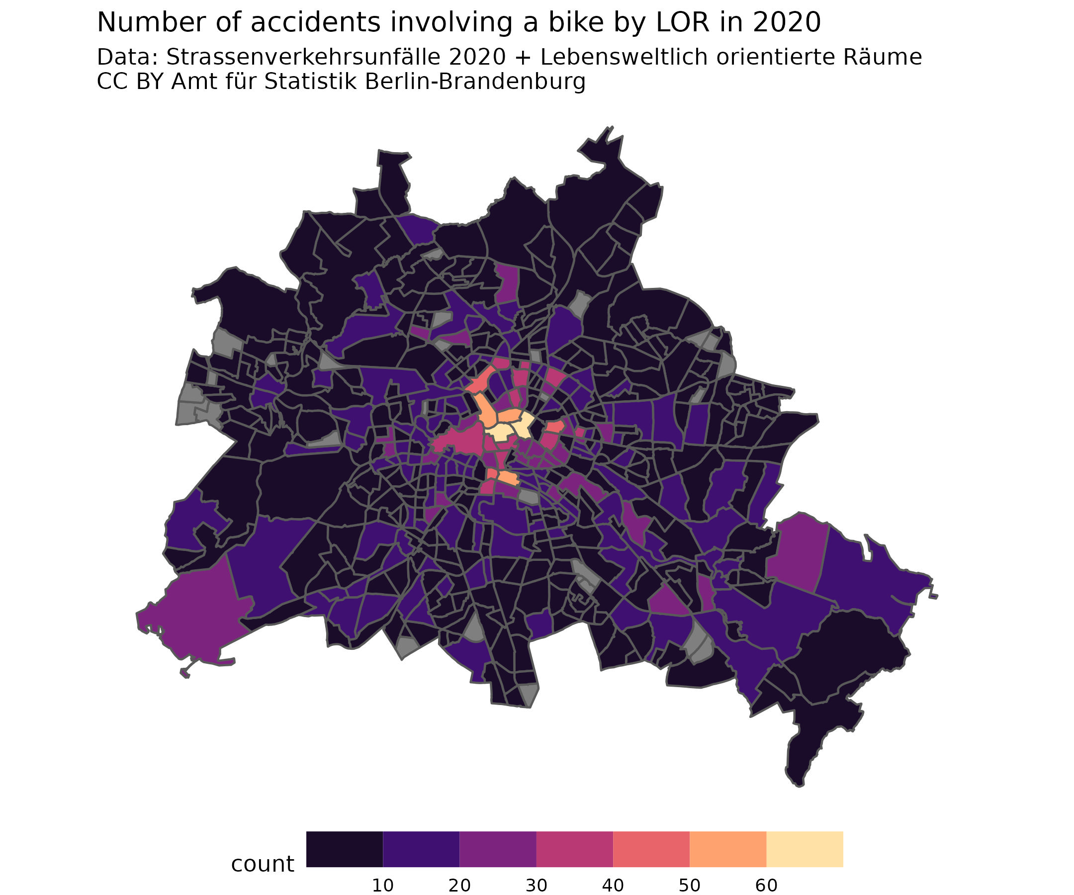
Map of accidents involving a bike by LOR in 2020. Without doubt, most of the accidents happened in the center of the city, where most of the biking activity happens. Plot made with r and ggplot2 of showing the accident in 2020 (data here).
Show the code of the exhibit
library(sf)library(dplyr)library(ggplot2)crash <-read.csv2("raw_data/AfSBBB_BE_LOR_Strasse_Strassenverkehrsunfaelle_2020_Datensatz.csv",colClasses =c(rep("character", 3),rep("factor", 9),rep("integer", 6),rep("factor", 1),rep("numeric", 4)))colnames(crash) |>tolower() ->colnames(crash)crash[13:18] <-sapply(crash[13:18] , as.logical)crash <-subset(crash, istrad ==TRUE)crash |>group_by(lor_ab_2021, bez) |>summarise(count =n()) -> crash_loredlor <-st_read("raw_data/lor_planungsraeume_2021.gml")colnames(lor)[1:6] |>tolower() ->colnames(lor)[1:6]lor$plr_id <- lor$plr_id |>as.factor()subset(lor, select=-bez) -> lorcrash_sf <-left_join(lor, crash_lored, by=c(plr_id ="lor_ab_2021"))ggplot(crash_sf ) +geom_sf(aes(fill = count), show.legend =TRUE) +scale_fill_viridis_b(option ="A", n.breaks =10) +theme_void() +theme(legend.key.width =unit(0.1, "npc"),legend.position="bottom") +labs(title ="Number of accidents involving a bike by LOR in 2020",subtitle ="Data: Strassenverkehrsunfälle 2020 + Lebensweltlich orientierte Räume \nCC BY Amt für Statistik Berlin-Brandenburg")ggsave("2022-03-09_bike_crash_lor.jpg", width=7.2, height=6,bg="white")# Top 10crash_sf[order(crash_sf$count, decreasing = T), c("plr_name", "count")] %>%head(10)
Berlin’s map of bike accident by LOR. Data: Strassenverkehrsunfälle nach Unfallort in Berlin 2020 + Lebensweltlich orientierte Räume − CC BY Amt für Statistik Berlin-Brandenburg
“Top” 10:
LOR name
sum of accidents
Alexanderplatzviertel
68
Unter den Linden
61
Oranienburger Straße
54
Charitéviertel
53
Urbanstraße
51
Friedenstraße
43
Rathaus Yorckstraße
43
Humboldthain Nordwest
42
Großer Tiergarten
40
Leipziger Straße
39
Show the code of the exhibit
library(sf)library(dplyr)library(ggplot2)crash <-read.csv2("raw_data/AfSBBB_BE_LOR_Strasse_Strassenverkehrsunfaelle_2020_Datensatz.csv",colClasses =c(rep("character", 3),rep("factor", 9),rep("integer", 6),rep("factor", 1),rep("numeric", 4)))colnames(crash) |>tolower() ->colnames(crash)crash[13:18] <-sapply(crash[13:18] , as.logical)crash <-subset(crash, istrad ==TRUE)crash |>group_by(lor_ab_2021, bez) |>summarise(count =n()) -> crash_loredlor <-st_read("raw_data/lor_planungsraeume_2021.gml")colnames(lor)[1:6] |>tolower() ->colnames(lor)[1:6]lor$plr_id <- lor$plr_id |>as.factor()subset(lor, select=-bez) -> lorcrash_sf <-left_join(lor, crash_lored, by=c(plr_id ="lor_ab_2021"))ggplot(crash_sf ) +geom_sf(aes(fill = count), show.legend =TRUE) +scale_fill_viridis_b(option ="A", n.breaks =10) +theme_void() +theme(legend.key.width =unit(0.1, "npc"),legend.position="bottom") +labs(title ="Number of accidents involving a bike by LOR in 2020",subtitle ="Data: Strassenverkehrsunfälle 2020 + Lebensweltlich orientierte Räume \nCC BY Amt für Statistik Berlin-Brandenburg")ggsave("2022-03-09_bike_crash_lor.jpg", width=7.2, height=6,bg="white")# Top 10crash_sf[order(crash_sf$count, decreasing = T), c("plr_name", "count")] %>%head(10)