‘Top’ 10 most dangerous neighborhoods (for street users)
Berlin
Bike
2022
Open Data
Author
Néhémie Strupler
Published
March 7, 2022
Yesterday’s post was about the repartition of the sum of accidents by LOR. Having a basic idea of the data, we can marge them to the 2021’s LOR division (see this note).
Picture of the day
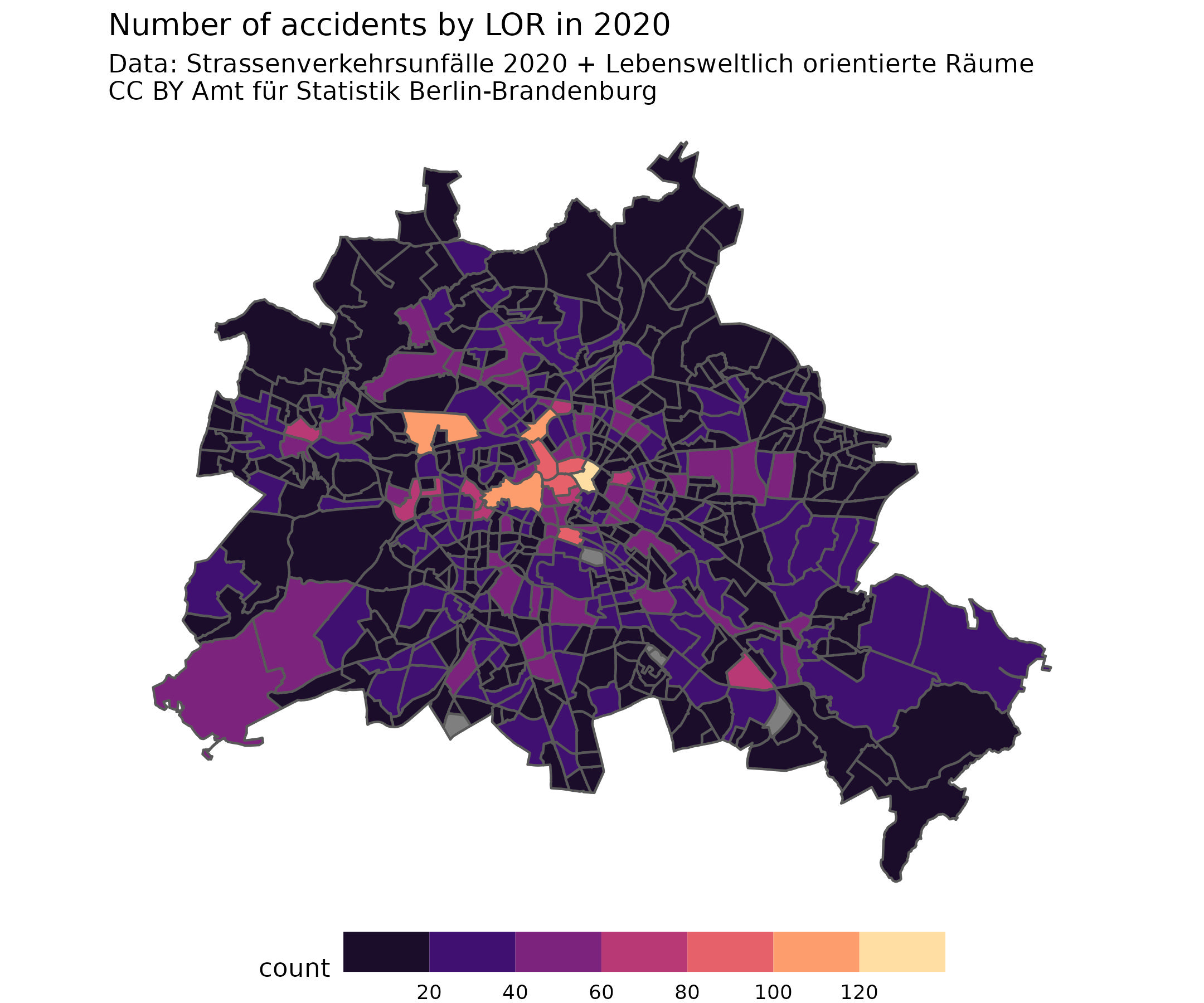
Map of accidents by LOR in 2020 coloured by the sum of accidents. Most of the accidents happen in the center of the city with some outliers. Plot made with r and ggplot2 of showing the accident in 2020 (data here).
Show the code of the exhibit
library(sf)library(dplyr)library(ggplot2)crash <-read.csv2("raw_data/AfSBBB_BE_LOR_Strasse_Strassenverkehrsunfaelle_2020_Datensatz.csv",colClasses =c(rep("character", 1),rep("factor", 12),rep("integer", 6),rep("factor", 1),rep("numeric", 4)))crash[14:19] <-apply( crash[14:19], 2, as.logical)colnames(crash) |>tolower() ->colnames(crash)crash |>group_by(lor_ab_2021, bez) |>summarise(count =n()) -> crash_loredlor <-st_read("raw_data/lor_planungsraeume_2021.gml")colnames(lor)[1:6] |>tolower() ->colnames(lor)[1:6]lor$bez <- lor$bez |>as.factor()lor$plr_id <- lor$plr_id |>as.factor()crash_sf <-left_join(lor, crash_lored, by=c(plr_id ="lor_ab_2021"))jpeg("2022-03-07_crash_sf.jpg",width=1200, height=1000, quality=90,res=120)ggplot(crash_sf ) +geom_sf(aes(fill = count), show.legend =TRUE) +scale_fill_viridis_b(option ="A", n.breaks =10) +theme_void() +theme(legend.key.width =unit(0.1, "npc"),legend.position="bottom") +labs(title ="Number of accidents by LOR in 2020",subtitle ="Data: Strassenverkehrsunfälle 2020 + Lebensweltlich orientierte Räume \nCC BY Amt für Statistik Berlin-Brandenburg")dev.off()
Data: Strassenverkehrsunfälle nach Unfallort in Berlin 2020 + Lebensweltlich orientierte Räume − CC BY Amt für Statistik Berlin-Brandenburg